Proposed by Mohamed Wahbi

Overview

The general definition of the SensorDisCSP family is as follows:

The target tracking in distributed sensor network problem (SensorDisCSP) is a real distributed resource allocation problem. This problem consists of a set of $n$ stationary sensors, $\mathcal{S} = \{s_{1}, \ldots, s_{n}\}$, and a set of $m$ targets, $\mathcal{T} = \{t_{1}, \ldots, t_{m}\}$, moving through their sensing range. The objective is to track each target by sensors. Thus, sensors have to cooperate for tracking all targets. In order for a target to be tracked accurately, at least three sensors must concurrently turn on overlapping sectors. This allows the target’s position to be triangulated. However, each sensor can track at most one target. Hence, a solution is an assignment of three distinct sensors to each target.

A solution must satisfy the visibility and the compatibility constraints. The visibility constraint defines the set of sensors to which a target is visible. This mainly depends on the sensing range of each sensor and to the presence of obstacles in the sensing range. The sensing ranges of all sensors form a sensing graph. The compatibility constraint defines the compatibility among sensors (sensors within the communication range of each other). There may be obstacles or noise sources on the communication area leading to breaking links of communication. The compatibility constraints are represented through the communication network.

Grid Model

The Grid-based SensorDisCSP (or GSensorDisCSP, for short) is a specific variant of the general SensorDisCSP: as before, we have multiple sensors $\mathcal{S} = \{s_{1}, \ldots, s_{n}\}$, multiple objects/tagets $\mathcal{T} = \{t_{1}, \ldots, t_{m}\}$ which are to be tracked by the sensors subject to visibility and compatibility constraints, and the goal is to allocate three sensors to track each object/target, while keeping these triplets of sensors pair-wise disjoint. However, in GSensorDisCSP the sensors are located on the nodes of a uniform grid of $n$ nodes, and the target objects are located within the surface enclosed by the grid (i.e., the grid specifies the generally trackable region).

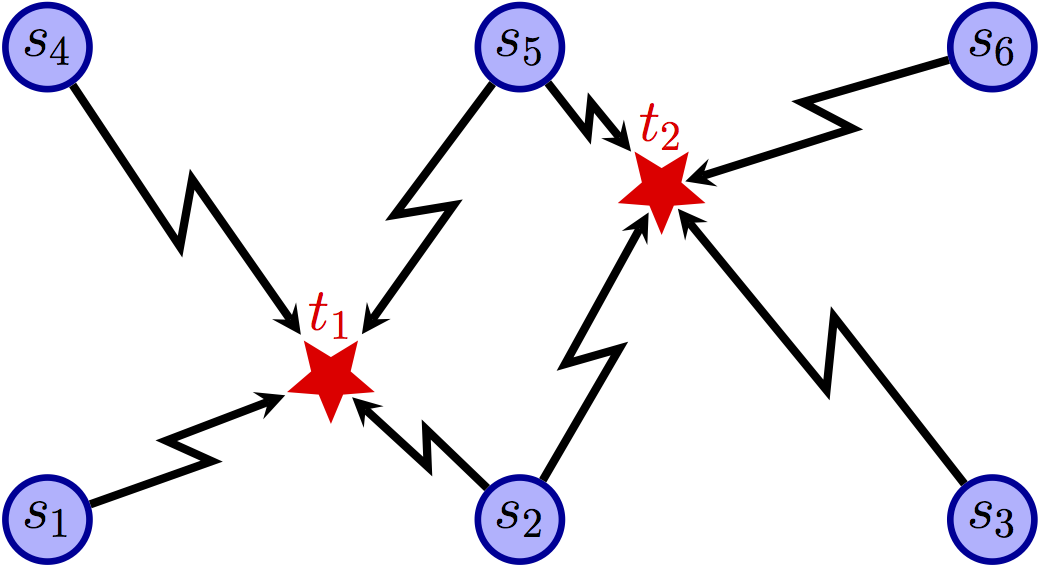
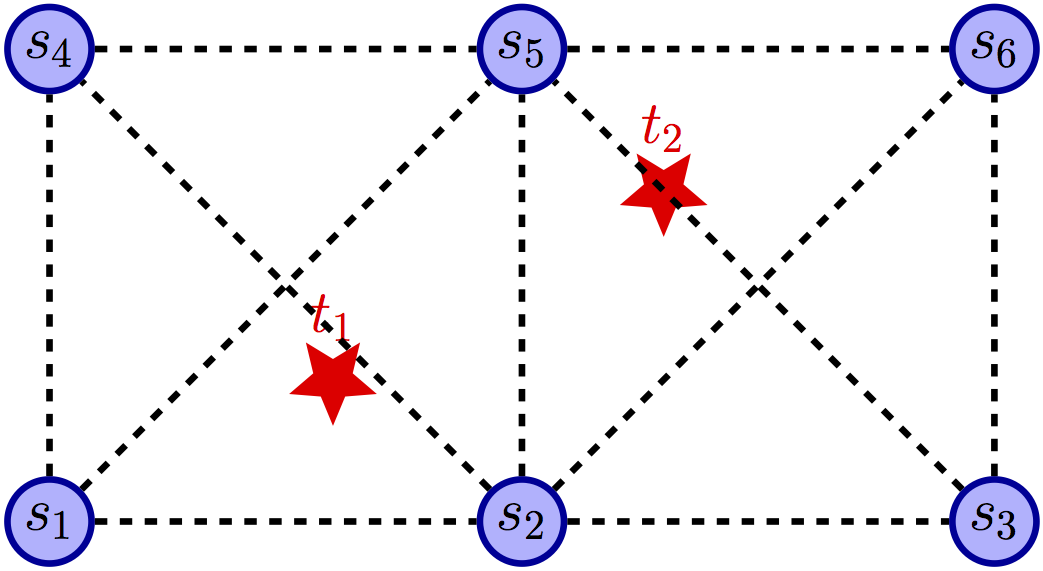
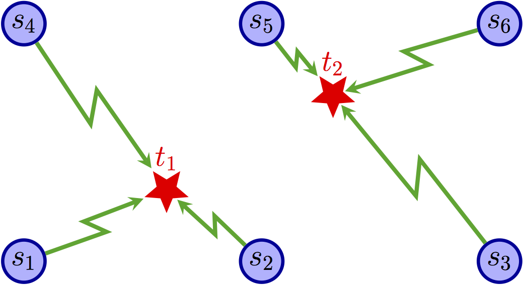
Fig.1 shows an example of the target tracking problem in distributed sensor networks where $s_{i}$ represents the sensor and $t_{j}$ represents the target. In this example sensors are arranged on the nodes of a uniform grid and it is assumed that only one target can exist in one area. This instance consists of 2 targets: $t_{1}$ and $t_{2}$ and 6 sensors: $s_{1}$, $\ldots$, and $s_{6}$. Each target has a set of sensors that can possibly detect it (the sensors in the nodes of the area where the target is located), as depicted by the bipartite sensing graph in Fig.1(a). For example, $t_{1}$ can be tracked by $s_{1}$, $s_{2}$, $s_{4}$, and $s_{5}$. In addition, it is required that each target be assigned three sensors that satisfy a compatibility relation with each other; this compatibility relation is depicted by the communication network in Fig.1(b). Each sensor can communicate with all sensors that are at most 1 hop (rectilinear and/or diagonal) from it. Finally, it is required that each sensor only track at most one target. A possible solution is depicted in Fig.1(c), where the set of three sensors assigned to each target is indicated by the green edges.

Distributed CSP Formulation

In the following, three Distributed CSP based formalizations for target tracking in sensor network problem are shown. These are TaV, STaV and SaV.

Target as Variable (TaV):

Target as Variable (TaV) is a model of formalization which defines an agent for each target (i.e., the set of agent is exactly the set of targets $\mathcal{A}=\mathcal{T}$). There are three variables per agent, one for each sensor that we need to allocate to the corresponding target. The domain of each variable is the set of sensors that can detect the corresponding target (the visibility constraint defines such sensors). The inter-agent constraints between the variables of one agent (target) specify that the three sensors assigned to the target must be distinct.

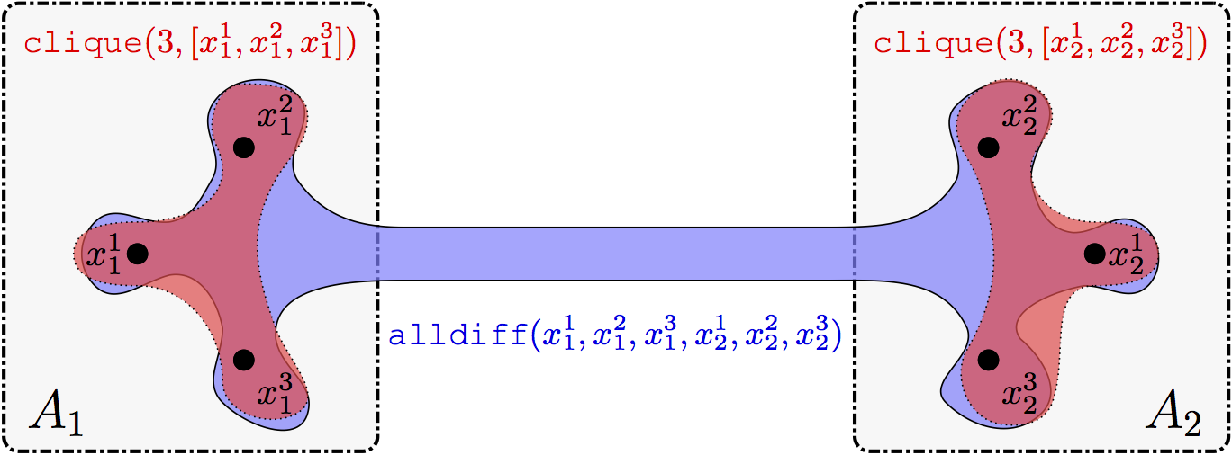
In Fig. 2, the instance of target tracking in distributed sensor network shown in Fig. 1 is formalized as a TaV problem. Each target is represented by an agent, i.e., there is two agents $A_{1}$ representing $t_{1}$ and agent $A_{2}$ representing $t_{2}$. Each agent controls 3 distinct variables (one for each sensor to track the target). Agent $A_{1}$ has variables $x_{1}^{1}$, $x_{1}^{2}$, and $x_{1}^{3}$, while agent $A_{2}$ has variables $x_{2}^{1}$, $x_{2}^{2}$, and $x_{2}^{3}$. The domain of variables of each agent is the set of sensors that can track the target represented by the that agent. Target $t_{1}$ can be tracked by $s_{1}$, $s_{2}$, $s_{4}$, and $s_{5}$, thus, $D_{1}^{1}=D_{1}^{2}=D_{1}^{3}=\{1,2,4,5\}$. For agent/target $A_{2}/t_{2}$, $D_{2}^{1}=D_{2}^{2}=D_{2}^{3}=\{2,3,5,6\}$. The domains are used to represent the visibility constraint. There is a $\texttt{clique}$ constraint between variables of each agent: $\texttt{clique}(3,[x_{1}^{1},x_{1}^{2},x_{1}^{3}])$ (respectively $\texttt{clique}(3,[x_{2}^{1},x_{2}^{2},x_{2}^{3}])$) specifying that there is a maximum clique of size 3 in the communication graph between sensors assigned to target $t_{1}$ (respectively $t_{2}$). $\texttt{clique}$ constraint is used for representing the compatibility constraint. An $\texttt{allDiff}$ constraint on the variables of agents having a common sensor in there domains is used to specify that each sensor can track at most one target: $\texttt{allDiff}(x_{1}^{1},x_{1}^{2},x_{1}^{3},x_{2}^{1},x_{2}^{2},x_{2}^{3})$.

A solution (Fig.1(c)) to that problem is: $x_{1}^{1}=1,x_{1}^{2}=2,x_{1}^{3}=4,x_{2}^{1}=3,x_{2}^{2}=5,x_{2}^{3}=6$.

Sensor-Target as Variable (STaV):

Sensor-Target as Variable (STaV) is a model of formalization which defines a variable for a pair of a sensor and a target. Each sensor $s_{i}$ is modeled by an agent $A_{i}$. For each agent $A_{i}$ there is a binary variable $x_{i}^{j}$ (i.e., $D_{i}^{j}=\{0,1\}$) for each target $t_{j}$ that can be tracked by $s_{i}$. For each sensor, there is a constraint specifying that it can not track more than one target: $\forall s_{i}\in\mathcal{S},\sum_{j=1}^{m}{x_{i}^{j}}\leq 1$. For each target, there is a constraint specifying that it must be tracked by at least 3 sensors: $\forall t_{j}\in\mathcal{T},\sum_{i=1}^{n}{x_{i}^{j}}\geq 3$.

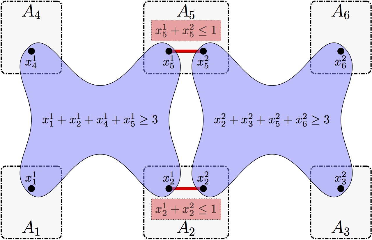
An example of a sensor network shown in Fig. 1 is formalized as a STaV problem shown in Fig. 3. In Fig. 3, $x_{i}^{j}$ represents a variable of $s_{i}$ for target $t_{j}$. For each sensor $s_{i}$, variables are defined for targets that can be observed by $s_{i}$. In this example, $A_{1}$, $A_{3}$, $A_{4}$, and $A_{6}$ have one variable each because they represent sensors that can observe only one target ($t_{1}$ for $s_{1}$ and $s_{4}$ and $t_{2}$ for $s_{3}$ and $s_{6}$). $s_{2}$ and $s_{5}$ have two variables because they can observe two targets (i.e., $t_{1}$ and $t_{2}$). A value of $x_{i}^{j}$ represents which sensors are allocated to $t_{j}$. We have 4 constraints in that problem where constraints $c_{1}$ and $c_{2}$ specifying that a sensor can track at most one target and constraints $c_{3}$ and $c_{4}$ specifying that a target must be tracked by at least 3 sensors.

• $c_{1}: x_{2}^{1}+x_{2}^{2}\leq 1$
• $c_{2}: x_{5}^{1}+x_{5}^{2}\leq 1$
• $c_{3}: x_{1}^{1}+x_{2}^{1}+x_{4}^{1}+x_{5}^{1}\geq 3$
• $c_{4}: x_{2}^{2}+x_{3}^{2}+x_{5}^{2}+x_{6}^{2}\geq 3$

A solution (Fig.1(c)) to that problem is: $x_{1}^{1}=1,x_{2}^{1}=1,x_{2}^{2}=0,x_{3}^{2}=1,x_{4}^{1}=1,x_{5}^{1}=0,x_{5}^{2}=1,x_{6}^{2}=1$.

Sensors as Variable (SaV):

Sensor as Variable (SaV) is a model of formalization which defines an agent $A_{i}$ for each sensor $s_{i}$. For each agent/sensor $A_{i}$ there is one single variable $x_{i}$. The domain of a variable $x_{i}$ is defined by the set of targets that sensor $s_{i}$ can track. There is an $\texttt{atleast}$ constraint on the variables $[x_{i},…,x_{k}]$ that can track each target, i.e., $\forall t_{j}\in\mathcal{T},\texttt{atleast}(3,[x_{i},\ldots,x_{k}],j)$ such that $\forall x_{l}\in [x_{i},\ldots,x_{k}]$, $j\in D_{l}$.

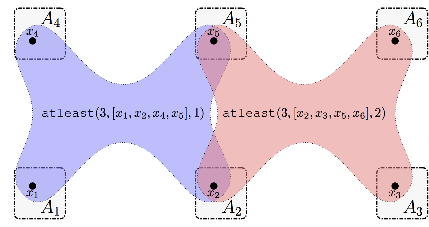
An example of a sensor network shown in Fig. 1 is formalized as a SaV problem shown in Fig. 4. In Fig. 4, each sensor $s_{i}$ is represented by a variable $x_{i}$ controlled by agent $A_{i}$. Thus, there is 6 variales/agents (i.e., $x_{1},\ldots,x_{6}$). The domain of each variable $x_{i}$ is the set of targets that $s_{i}$ can track. Thus, $D_{1}=D_{4}=\{1\}$, $D_{3}=D_{6}=\{2\}$ and $D_{2}=D_{5}=\{1,2\}$. There is 2 $\texttt{atleast}$ constraints (one for each target): $\texttt{atleast}(3,[x_{1},x_{2},x_{4},x_{5}],1)$ and $\texttt{atleast}(3,[x_{2},x_{3},x_{5},x_{6}],2)$ specifying that at least 3 sensors among $\{s_{1},s_{2},s_{4},s_{5}\}$ must track target $t_{1}$ and at least 3 sensors among $\{s_{2},s_{3},s_{5},s_{6}\}$ must track target $t_{2}$.

A solution (Fig.1(c)) to that problem is: $x_{1}=1,x_{2}=1,x_{3}=2,x_{4}=1,x_{5}=2,x_{6}=2$.